MNIST classifier

After finishing theIris classifier, and part of link title Andrew Ng’s ML course, in which he talks about creating a Neural Network classifier to classify hand written digits I decided to try and write my own hand written digit classifier using Keras.

Git

https://github.com/Tzeny/mnist-classfier

Dataset

To train and test the model I used the MNIST dataset. If you are using Keras you can automatically download and import it1:

from keras.datasets import mnist

(x_train, y_train), (x_test, y_test) = mnist.load_data()

I used the above method.

Convolutional version

Unfortunately I did not use the same random seed for these experiments so take the results here with a grain of salt :(

Architecture	Accuracy on test set
2 conv layers w dropout	98.66%, 98.71%
2 conv layers w dropout w 2 dense	98.67 %
2 conv layers w/o dropout	98.60%, 98.59 %
1 conv layer w dropout	97.65 %
4 conv layer w dropout	98.8 % , 98.36 %
3 conv layer w dropout	98.95 % , 98.99 %
3 conv layer w dropout w 2 dense rmsprop	98.82 % , 98.72 %
3 conv layer w dropout w 2 dense sgd	99 %
3 conv layer w/o dropout w 2 dense sgd	99.0 %
3 conv layer dense drop dense drop dense sgd	99.11 %, 99.0 %, 99.11 %
4 conv layer dense drop dense drop dense sgd	99.14 %, 98.92 %
4 conv layer dense drop dense drop dense sgd (with activations right after conv layers)	99.36 %, 99.28 %
4 conv w act dsn dr dsn dr dsn sgd (w batch normalization)	99.58 %, 99.39 %, 99.33 %
4 conv w act dsn dr dsn dr dsn dr sgd (w batch normalization)	99.35 %, 98.94 %
4 conv w act dsn dr dsn dr dsn dr sgd (w batch normalization + l2 regularization)	97.34 %, 98.68 %
4 conv w act dsn dr dsn dr dsn dr sgd (w batch normalization + l1 regularization)	87.51 %, 79.44 %

Source code for CNN version: https://tzeny.ddns.net:4430/Tzeny/udemy-zero-to-deep-learning/blob/master/course/MnistConv.ipynb

Preprocessing the dataset

When you import the dataset, x_train is a 3D matrix of shape (60000,28,28) and x_test is a 3D matrix of shape (10000,28,28). I reshaped them into 2D matrices of shapes (60000, 784) and (10000, 784) respectively.

Next we need to take the labels in the y_train and y_test vectors and map them to binary class matrices. For this we will use the to_categorial function from Keras2:

#dataset:
#   x_train 60000 28x28 uint8_encoded images
#   y_train 60000   [0-9] labels
#   x_test  10000 28x28 uint_8 encoded images
#   y_test  60000   [0-9] labels

#reshape our dataset to make it processable by the NN
x_train = np.reshape(x_train, (60000,784))
x_test = np.reshape(x_test, (10000, 784))

#create a vector with 10 rows for each value in y_train in y_test, to be used by our activation layer
y_train_labels = keras.utils.to_categorical(y_train, num_classes=10)
y_test_labels = keras.utils.to_categorical(y_test, num_classes=10)

Full code

import matplotlib.pyplot as plt
import numpy as np

import keras
from keras.models import Sequential
from keras.layers.core import Dense, Activation, Dropout
from keras.utils import plot_model
from keras.datasets import mnist

import time
from datetime import datetime


max_epoch=50
optimizer='adam'
dropout_ratio = 0.2
neurons_in_layers = 64
#will be used to give all
date = time.strftime('%Y-%m-%d-%H:%M')

#load dataset
(x_train, y_train), (x_test, y_test) = mnist.load_data()

#dataset:
#   x_train 60000 28x28 uint8_encoded images
#   y_train 60000   [0-9] labels
#   x_test  10000 28x28 uint_8 encoded images
#   y_test  60000   [0-9] labels

#reshape our dataset to make it processable by the NN
x_train = np.reshape(x_train, (60000,784))
x_test = np.reshape(x_test, (10000, 784))

#create a vector with 10 rows for each value in y_train in y_test, to be used by our activation layer
y_train_labels = keras.utils.to_categorical(y_train, num_classes=10)
y_test_labels = keras.utils.to_categorical(y_test, num_classes=10)

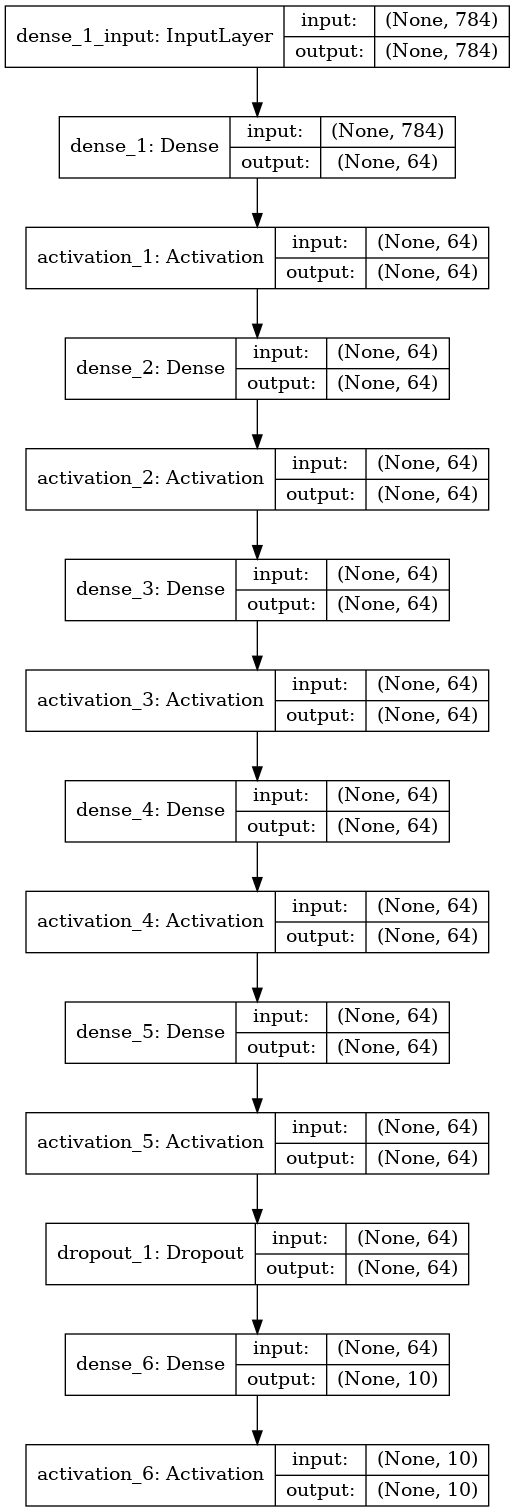
model = Sequential([
    Dense(neurons_in_layers, input_shape=(784,)),
    Activation('relu'),
    Dense(neurons_in_layers),
    Activation('relu'),
    Dense(neurons_in_layers),
    Activation('relu'),
    Dense(neurons_in_layers),
    Activation('relu'),
    Dense(neurons_in_layers),
    Activation('relu'),
    Dropout(dropout_ratio),
    Dense(10),
    Activation('softmax'),
])

model.compile(loss='categorical_crossentropy', optimizer=optimizer, metrics=['accuracy'])

plot_model(model, to_file="models-png/" + date + '_model.png',  show_shapes=True)

history = model.fit(x_train, y_train_labels, validation_data=(x_test, y_test_labels), epochs=max_epoch, verbose=1)

#save model
model.save_weights("models/" + optimizer + "_opt-" + str(max_epoch) + "_eps-" + date + ".h5")
print("Saved model to disk")

#plot data

# list all data in history
print(history.history.keys())

# summarize history for accuracy
plt.plot(history.history['acc'])
plt.plot(history.history['val_acc'])
plt.plot(history.history['loss'])
plt.plot(history.history['val_loss'])

# plot 3 so that we can better see our model's accuracy
plt.axhline(y=1, color='g', linestyle='--')
plt.axhline(y=0.95, color='orange', linestyle='--')
plt.axhline(y=0.9, color='r', linestyle='--')

plt.title('model - accuracy and loss')
plt.ylabel('accuracy/loss')
plt.xlabel('epoch')
plt.legend(['train_acc', 'test_acc', 'train_loss', 'val_loss'], loc='upper left')

plt.savefig(optimizer + "_opt-" + str(max_epoch) + "_eps-" + date +'_score.png', bbox_inches='tight')
print("Saved plot to disk")

Displaying the result

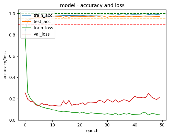
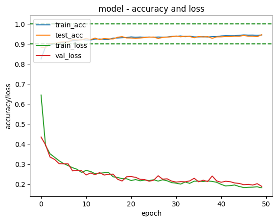
In order to display the result I took an online piece of code3 and modified it to plot training accuracy, test set accuracy, training loss and test loss and then save them to a file.

Model used to get above results

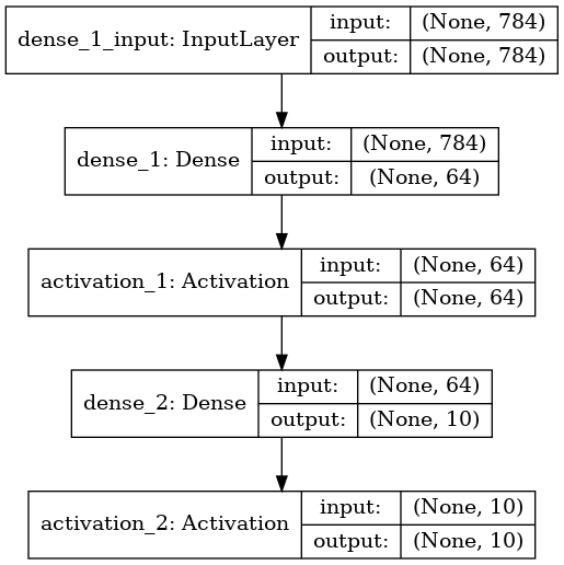
Try other architectures

The problem with this is that it has started overfitting the test set.