Types of Machine Learning algorithms

Based on the Coursera Machine Learning course1

Some more detailed information: https://docs.google.com/document/d/11i46PW6rc0sYrQ8nQ5tqCtXwvR09TiOu8M3-M-K_PUQ/edit?usp=sharing

Supervised Learning

Regression problem

We choose a model class: y=f(x;W) - a model class f is a way of using some numerical parameters W, to map each input vector x into a predicted output y

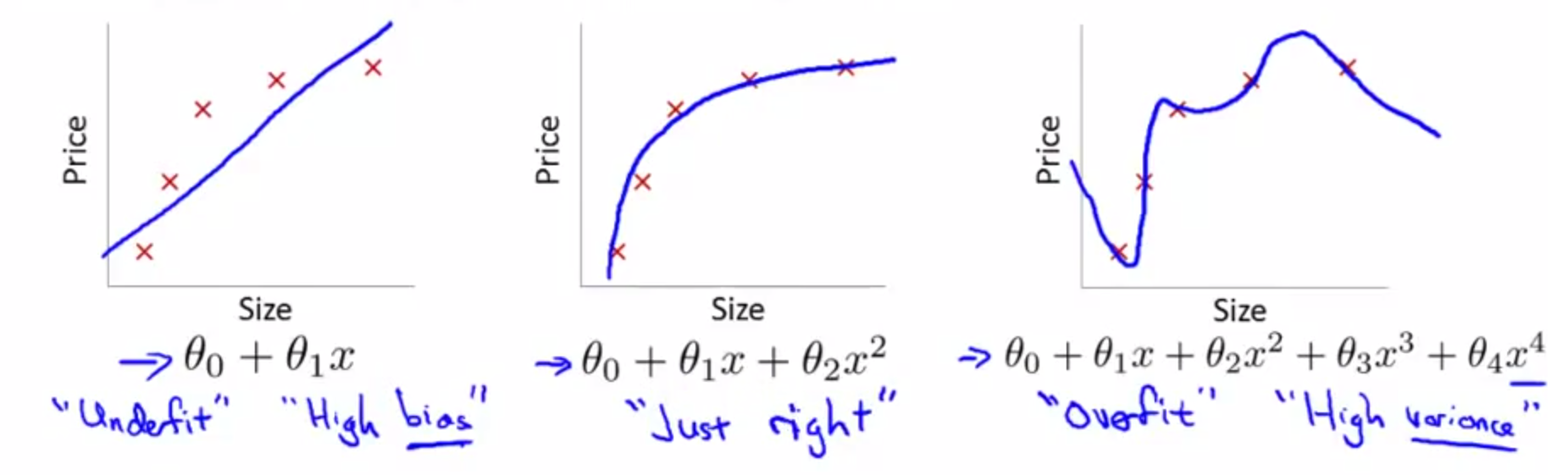
Univariate linear regression:

• Prediction: h**θ(x)=θ0 + θ1 * x
• Cost function: $J(\theta_0,\theta_1) = \sum_{i=1}^m(h_\theta(x^{(i)})-y^{(i)})^2$

Multivariate linear regression:

• Prediction: hθ*(*x*)=*θ*0 * *x*0 + *θ*1 * *x*1 + … + *θn * x**n
• Cost function: $J(\theta_0,\theta_1) = \sum_{i=1}^m(h_\theta(x^{(i)})-y^{(i)})^2$

Classification problems

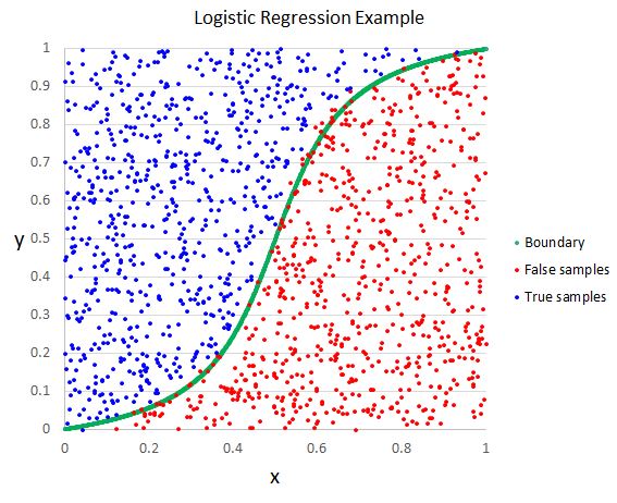
Y={0,1} - binary classification; can have more values We end up creating a decision boundary; inside we predict y=1, outside we predict y=0

Logistic regression with 2 outputs (binary classification):

• Prediction: $h_\theta(x)=g(\Theta^T*x)=\frac{1}{1+e^{-\Theta^T*x}}$ (sigmoid/logistic function)
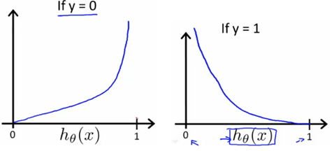
• Cost: $J(\theta) = -\frac{1}{m}\sum_{i=1}^m(y^{(i)}*\log(h_\theta(x^{(i)}) + (1-y^{(i)})*\log(1-h_\theta(x^{(i)})) + \frac{\lambda}{2m}\sum_{j=1}^n\theta_j$

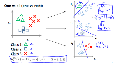
Logistic regression with n outputs (one vs all algorithm):

If we have to distinguish between many similar classes (ex: dog breeds), the problem is called fine grained classification.

Support vector machines

They are learning algorithms used for binary classification of data. What a SVM does is represent examples as points in space separated by as wide a margin as possible. New examples are mapped in the same space and depending on which side of the boundary they fell are classified into 2 categories.

It can use Kernels, which take a number of landmarks in space and use the distance between an example X and a landmark L as a feature in the hypothesis. There are multiple ways to compute the distance:

• Gaussian distance: $f1 = similarity(x,l) = \exp(-\frac{

• Polynomial kernel
• String kernel
• etc

Usually when we train we use each of the train examples as a landmark.

Cost function: $C\sum_{i=1}^m[y^{(i)}cost_1(\theta^T*f^{i})+(1-y^{(i)})cost_0(\theta^T*f^{i})] + \frac{1}{2}\sum_{j=1}^m \theta_j^2$

Large C -> lower bias, higher variance Small c -> higher bias, lower variance

Largeσ2 -> features fi vary more smoothly -> higher bias, lower variance Smallσ2 -> features fi vary less smoothly -> lower bias, higher variance

Natural Language Processing

Natural language processing is an area of computer science and artificial intelligence concerned with the interactions between computers and human languages, in particular how to program computers to process and analyze large amounts of natural language data.

Unsupervised learning

We give our algorithm a set of unlabeled data and we ask it for example to find order in the data.

Recommender systems - content based

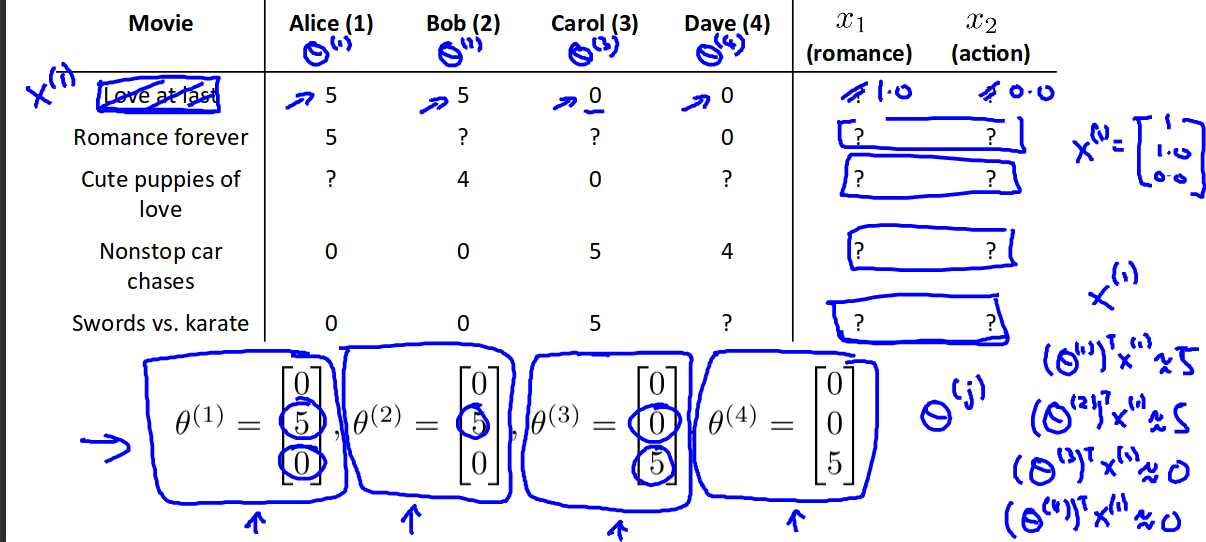
nu - number of users nm - number of movies r(i,j) = 1 if user i has rated movie j y(i,j) = rating given by user i to movie j (defined only if r(i,j)==1) θ^j = parameter vector for user j x^i = feature vector for movie i m^j = number of movies rated by user j to learn θ^j

For each user we learn a parameter vector θ^j of size nx1, and for each unrated movie i we predict user j will rate it (θ^j)’*x^i stars.

Optimization objective

$\underset{\theta^{(1)},\theta^{(2)},… \theta^{(n_u)}}{min}\frac{1}{2}\sum_{j=1}^{n_u}\sum_{i:r(i,j)=1}({\theta^{(j)}}^T*x^{(i)}-y^{(i,j)})^2+\frac{\lambda}{2}\sum_{j=1}^{n_u}\sum_{k=1}^n(\theta_k^{(j)})^2$

Gradient descent update

θk*(*j*) := *θk(j) − α∑i : r(i, j)=1(θ(j)T * x(i) − y(i, j))x**k(i)for k=0

θk*(*j*) := *θk(j) − α(∑i : r(i, j)=1(θ(j)T * x(i) − y(i, j))xk*(*i*) + *λθ**k(j))for k != 0

Collaborative filtering

The algorithm should learn a good set of features x^i on its own.

$\underset{x^{(i)}}{min}\frac{1}{2}\sum_{j=1}^{n_u}\sum_{i:r(i,j)=1}({\theta^{(j)}}^T*x^{(i)}-y^{(i,j)})^2+\frac{\lambda}{2}\sum_{k=1}^n(x_k^{(i)})^2$

Given θ^1, θ^2, … θ^nu learn x^1, x^2, …,x^nm

$\underset{x^{(1)},x^{(2)},… x^{(n_m)}}{min}\frac{1}{2}\sum_{j=1}^{n_m}\sum_{i:r(i,j)=1}({\theta^{(j)}}^T*x^{(i)}-y^{(i,j)})^2+\frac{\lambda}{2}\sum_{i=1}^{n_m}\sum_{k=1}^n(x_k^{(i)})^2$

Given a set of values for x^i we can estimate θ^j and vice versa.

Algorithm

1. Initializa x^1, x^2, …,x^nm and θ^1, θ^2, … θ^nu to random small values 2. Minimize J(x^1, x^2, …,x^nm; θ^1, θ^2, … θ^nu) using an optimization algorithm:

xk*(*i*) := *xk(i) − α(∑i : r(i, j)=1(θ(j)T * x(i) − y(i, j))xk*(*i*) + *λx**k(i))

θk*(*j*) := *θk(j) − α(∑i : r(i, j)=1(θ(j)T * x(i) − y(i, j))xk*(*i*) + *λθ**k(j))

For a user with parameters θ and a movie with (learned) features x predict rating θ^T*x.

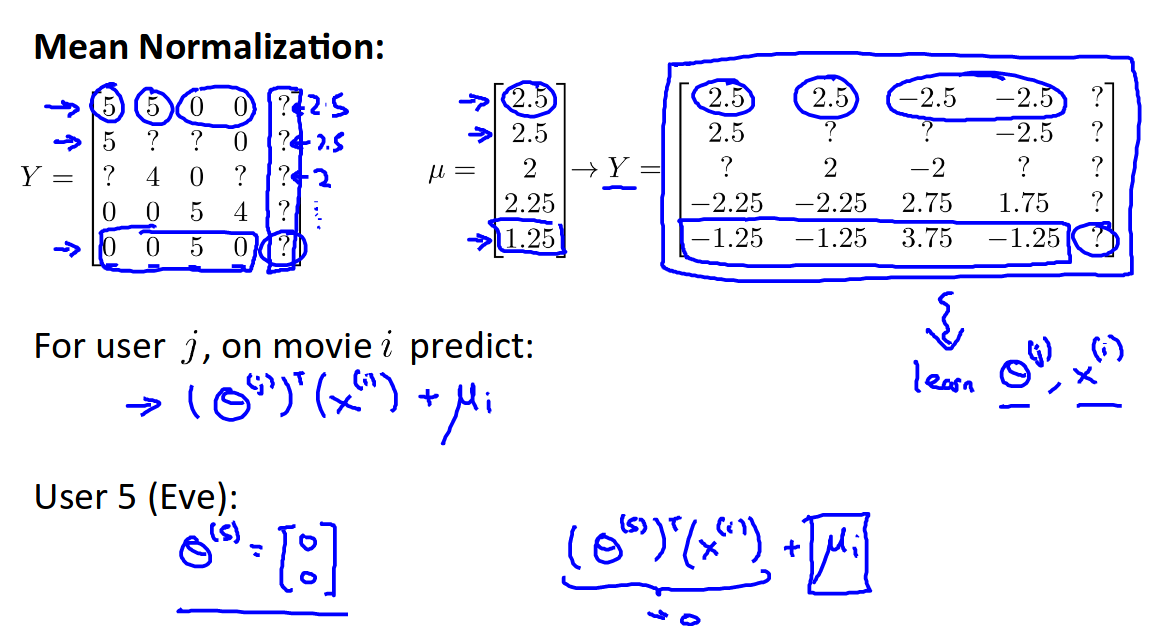
Mean normalization

Anomaly Detection

Given a set of features without labels, try to learn a way of finding out if new features are anomalous. Examples:

• given aircraft engine heat output and vibrations as features, and for new data points (new engines) determine the probability that they are defective
• given user’s actions on a website as features, determine the probability of an action being a fraud / suspicious
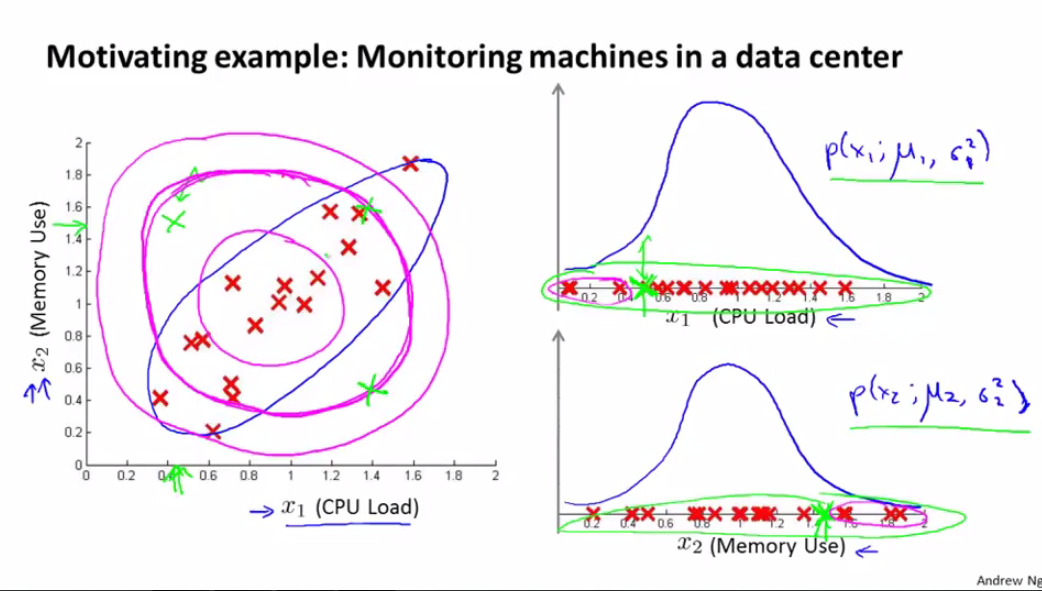
• given some metrics for computers in a cluster, determine the probability of something being wrong with one of the computers

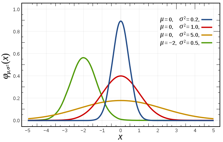
For this we can use the Gaussian distribution. We plot all features on the X axis, and we learn from them the parameters μ and σ^2. Then, we plot new examples onto the X axis and see how well they fit into the distribution. To find out μ and σ^ we use the following formulas:

$\mu_j=\frac{1}{m}\sum_{i=1}^mx_j^{(i)}$ $\sigma_j^2=\frac{1}{m}\sum_{i=1}^m(x_j^{(i)} - \mu_j)^2$

To compute the probability of a new example we use the following formula:

$\text{anomaly if }p(x) < \epsilon \text{ ; } p(x)=\prod_{j=1}^np(x;\mu_j,\sigma_j^2)=\prod_{j=1}^2\frac{1}{\sqrt{2\pi}\sigma_j}\exp{(-\frac{(x_j- \mu_j)^2}{2\sigma_j^2})}$

This algorithm can be combined with supervised learning. Suppose we have 10000 good examples, and 20 anomalous ones. We can split them up as follows:

• training set: 6000 good examples
• cross validation set: 2000 good, 10 anomalous - we can use this to choose ε
• test set: 2000 good, 10 anomalous

Non gaussian features

If we have features whose distribution is non gaussian we need to find ways to transform their distribution into a gaussian one (replace x with log(x), or sqrt(x)).

Adding new features

We can combine features to generate new features, that quantify relationships between existing features. For example, when monitoring a server we might come up with the feature: cpu_usage/network_traffic.

Multivariate Gaussian distribution

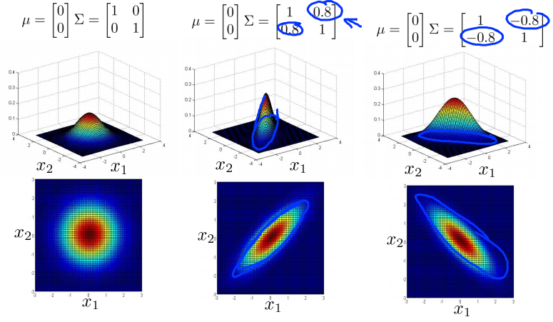
To capture the relationships between features we can opt to use one multivariate gaussian distribution instead of several gaussian distributions.

Fitting the parameters:

$\mu=\frac{1}{m}\sum_{i=1}^mx_j^{(i)}$ $\Sigma=\frac{1}{m}\sum_{i=1}^m(x^{(i)} - \mu)(x^{(i)} - \mu)^T$

Clustering

We give our algorithm a set of unlabeled data and ask it to find clusters of similar data points.

Motivation:

• Data compression: in the case of a large number of features (>100 for ex), we can use clustering to find related features, and combine them into new features, thus reducing the number of features
  • For instance we may have a feature that represents length in cm, and one that represents length in inches; we can combine these 2 features into a new feature z without losing much informations
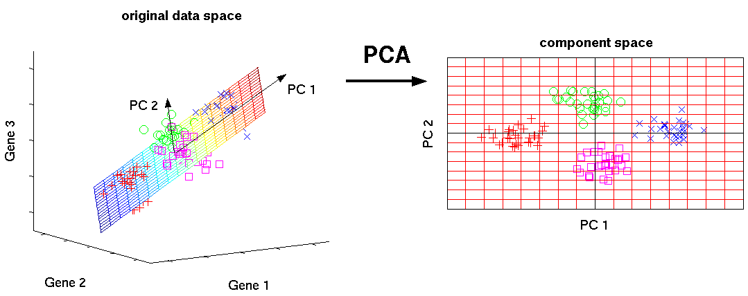
  • We can use dimensionality reduction to visualize your data, turning large number of features into 2 or 3 combined features

PCA - Principal Component Analysis

It can:

• Reduce disk space usage
• Speed up training time
• Help with visualisation

A method to reduce N dimensional data to K dimensions (K <= N)

It tries to find surfaces / vectors on which to project data points such that it minimizes the squared error of projection

To go from K back to N dimensions Xapproxn* * 1(*i*) = *Ureducen * k * z**k * 1(i)

Choosing K: [U,S,V] = svd(Sigma)

Pick the smallest K for which: $\frac{\sum_{i=1}^KS_{ii}}{\sum_{i=1}^NS_{ii}} \geq 0.99\text{ (variance retained)}$

We should use it only when necessary (data is taking up too much space, algorithm trains to slowly). It is not regularization! It is not linear regression!

K-Means algorithm

Is an iterative algorithm that uses a number of centroids: m to try and make sense of the data.

randomly initialize K cluster centroids:μ1, μ2…μK* ∈ *Rn

repeat for n iterations{
    #cluster assignment step which minimizes J with respect to c^(i), holding μk
    for i=1 to m
        c^(i) := index (from 1 to K) of closest cluster centroid

    #move centroid step which minimizes J with respect to μk, holding c^(i)
    for k=1 to K
        μk := average of all points assigned to cluster K
 }

If a cluster centroid ends up without any points assigned to it we can delete it (common) or randomly reinitialize it.

Random initialization

To initialize our centroids we will pick K random points from the dataset, and set our μ centroids at their positions. To make sure K-means doesn’t reach a local optima, especially for a small K, we will run the algorithm more than once.

Choosing K

We can use the elbow method, where we look at a plot of J versus K and choose based on how sharply the line turns.

You can choose depending on the downstream use of the data.

Reinforcement learning

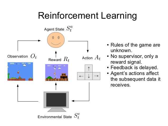
Here we have an agent and an environment which the agent can interact with. Based on his interactions and our goal, we give him a score. His goal is to optimize that score.

1. https://www.coursera.org/learn/machine-learning